Inhomogeneities and electrostatics
Having seen what the in-material cannot deliver and where the vacuum level's writ ends, we turn to what actually governs the spatial landscape inside materials. One of the main reasons these diagrams are powerful is that they clearly visualize devices with inhomogeneous composition and electric fields, that is, where is not flat. Typically all of this is conceived of as variations in , but lets us dig a bit more precisely into what is actually going on. This appendix collects the fine print: what a varying ladder really involves, why is not always a real electric field, and a catalog of everything that makes interfaces hard.
Two kinds of inhomogeneity
For a neutral solute, the standard-state level varies only where the medium itself varies, as in a graded composition; such variations are comparatively rare and slow to change. In a formal thermodynamic sense the are just more of the same, but pragmatically they vary far more readily. The extreme power of electrostatics means the react rapidly, and usually all together: within a fixed medium the whole ladder is slaved to the electrostatic potential,
Microscopically, obeys the Poisson equation , so if free charges accumulate anywhere then shifts, and every shifts along with it. Note that the quasi-neutral bulk does not mean ; in fact, very much not. As in basic electrostatics, the local-electroneutrality trick sends , forcing while freeing at every point to float to whatever value neutrality demands.
The difference between and : inhomogeneous electrostatics
That single- picture assumed a fixed, homogeneous medium, and it fails exactly where things get interesting. For a macroscopic description we separate the dipolar polarization charge off into a displacement field, leaving
However, the first equation only defines as "everything but polarization bound charge", and the second is only a valid constitutive relation inside a homogeneous medium.
It helps to split , where sums our local mobile carriers, and is static charge: dopants, the "fixed oxide charge" at the silicon/silicon-oxide interface, charged dislocations and grain boundaries, and sheet charges at interfaces generally. Even though these are fixed charges, we don't model them as "bound charges" in the normal (polarization) sense, since they need not come along with any compensating charge.
In an inhomogeneous region, the constitutive relation must generalize as well:
The built-in displacement is nonzero at interfaces (a sharp, delta-function dipole layer), through graded media, and (more subtly) wherever a nonideal solution carries concentration gradients, because there it is the activity convention that dictates how varies (a caveat the nonideality topic owns). Crucially, depends on how we defined in the first place: adopt a different convention and a compensating appears to soak up the change. In other words, is not always a real electric field. (There are even materials where a bulk polarization ambiguity lets be nonzero throughout the material, not just at its boundaries!)
The hillium–mountainium junction makes this concrete. There, stepped at an interface between two chemically identical liquids, so acquired a violent spike that no ion feels; and since the physical vanishes everywhere in that system, must contain the exact opposite spike. The fictitious field and its cancelling partner are two entries of one bookkeeping identity, and both evaporate under a different choice of smoothing.
Is the electric field real?
That subjectivity of sounds like a disaster for electromagnetism, yet notice what survives: the field is subjective, the split between and is subjective, and the total is unaffected by any of it. This "agree on , disagree on " is an interesting backwards twist on the usual polarization ambiguity, where everyone agrees on but the separation of charge into bound and free (and hence ) is ambiguous; I don't think the two are related. The practical upshot: on large scales we ignore by leaning on quasi-neutrality, while right at interfaces there is no honest way to reduce the physics to a naive , which is part of why interfaces get their own laws.
Maxwell's equations weather all of this, because only the curl of carries any direct weight: you may add an arbitrary conservative field to and, as long as , , and are untouched, nothing observable moves. The usual argument for the reality of (and ) comes from the Lorentz force, but this argument breaks inside of media: we know for example that in graded-bandgap heterostructures, we get a different field for electrons and holes! You can appeal to the Lorentz force on ghostly test charges to resolve this, but then you get back to the question of exactly how those test charges should sit inside the material. Yes, you can insist on a true by taking the smoothed average of under the microscope, which means will be the smoothed-out microscopic field , but this does not even win you any favour from the Maxwell equations.
Graded media and quasi-electric fields
A graded medium is an interface smeared into a continuum: the composition, and with it the whole standard-state ladder , varies smoothly across an extended region rather than jumping at a sharp plane. Everything from the previous section now happens in the bulk. Because the of different species depend differently on the local composition, they need not slope together, and each carrier ends up feeling its own quasi-electric field .
This is Kroemer's insight from graded-bandgap semiconductors (the heterojunction bipolar transistor being the famous case): the quasi-fields for different carriers are independent, they can differ in magnitude and direction, and none of them need equal the electrostatic .[1] A graded composition is, in this sense, a genuinely new kind of force on carriers, not reducible to any single field.
There is a further wrinkle specific to semiconductors. Our electron standard state is pinned to the band edge at its effective density of states , and in a graded material (and for holes) vary along with everything else. The drift-diffusion decomposition then splits into three pieces rather than two: the quasi-field , the familiar Fickian term, and a term in from the sliding reference concentration. Consider a flat band edge with a graded effective mass: at equilibrium the electrons pile up where states are plentiful (), and the ordinary diffusion term would read that pile-up as a current. The term exists to cancel exactly that mistake. Meanwhile never split anything and needs no correction.
The electrochemical version is a compositionally graded mixed ionic-electronic conductor, say a doping-graded ceria in which both oxide ions and electrons are mobile. Across the graded slab the electronic level and the ionic level slope at different rates, so electrons and oxide ions are pushed by different quasi-fields while is a third, separate slope.
One thing worth stating plainly: a fast solid-ion conductor is a concentrated, strongly nonideal medium, so the placement of the levels themselves inherits the single-ion activity ambiguity we keep running into. That is less a defect of the example than the whole point of this topic. The graded solid is exactly where the standard-state ladder, the per-carrier quasi-fields, and the activity conventions all turn subtle at once, and where reading everything off the traces rather than off matters most.
Homage to Kroemer's graded-bandgap picture, in ionic form: across a compositionally graded MIEC, the electronic level and the ionic level slope in opposite directions, a push no single electrostatic field could give two like-signed carriers, while the electrostatic is a third, separate slope. No single field describes all the carriers.
Beyond the simple case: the catalog
In basic electrostatics we described an incredibly elementary form of screening: an ideal homogeneous linear dielectric medium with a nice ideal dependence of charge carrier accumulation on , which led to relatively trivial results like the Poisson–Boltzmann screening equation. In general, electrostatics is a far harder problem. What follows is a deliberately non-exhaustive catalog of the main complications, grouped by kind:
- Interfaces are hard to pin down. Even for a simple interface (an electrode or heterojunction), fixing the value of the offset from first principles is hard; the "vacuum contact" / contact-potential-difference rule of thumb is notoriously unreliable in semiconductors. Real interfaces are also patchy and non-planar (electrostatics is fundamentally three-dimensional, and even 'planar' interfaces are microscopically irregular), and they can carry built-in monopolar charges, whether static and dopant-like (fixed oxide charge at the interface) or interface-specific (metal-induced gap states, electronic surface states, specific ion adsorption).
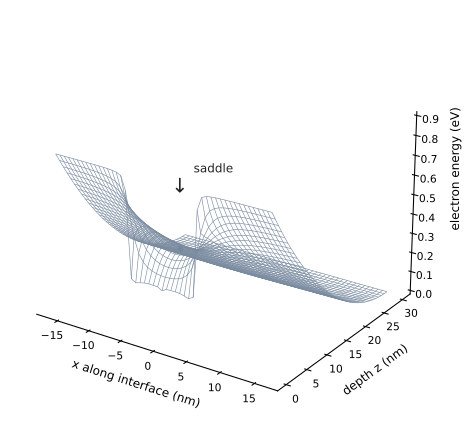
The first item drawn: in front of an interface whose barrier height varies from patch to patch, the potential is a genuinely three-dimensional Laplace problem. A low-barrier patch sits in a saddle point walled in by its higher-barrier surroundings (R. Tung's "pinch-off": Figs. 15–18 of his Schottky-barrier review), so the junction behaves like no single one-dimensional barrier at all.
- Nano geometry: very thin conductors (such as a graphene 2D electron gas) can only screen and conduct in two dimensions while electrostatics remains three-dimensional, so they have no quasi-neutral bulk and are 'all interface'.
- Breakdown of the local linear continuum: at very short ranges both charge density and can get nonlocal (a Fermi gas gets Friedel oscillations; ions get pair correlations; the solvent has a correlation length and 'overscreening'); at high fields the solvent's dielectric response is nonlinear (dielectric saturation), and it tends to set in under the same double-layer conditions where the nonlocal effects also appear, so it becomes a real mess; and where small scales and strong driving combine, itself can become ill-defined or need further refinement in meaning.
Takeaways
In the bulk, quasi-neutrality spares us from almost all of this: the ladder acts as a mere neutralizer, and the diagrams stay simple. The difficulty concentrates at interfaces, in graded and nonideal media, and at small scales, exactly where splinters into per-species quasi-fields and even loses its objectivity. The themselves remain well defined through all of it, and that is the point of building on them.
NEXT TOPIC: Standard state data
H. Kroemer, Nobel Lecture (2000), "Quasi-electric fields and band offsets: teaching electrons new tricks." The striking semiconductor version is that a graded gap can drive electrons and holes in the same direction, which no electrostatic field can do. ↩︎