under the microscope
When I came up with these band diagrams, it quickly became apparent that it is possible to entirely avoid invoking the electrostatic potential . This was not surprising given my semiconductor physics background, yet this is so dissonant with being so fundamental in the usual electrochemistry analysis. Digging a little bit deeper, however, we find that the theoretical electrochemists are already uncomfortable with the unmeasurable , and sometimes have argued to abolish entirely. This dates back to Guggenheim's 1929 and 1930 papers, and even earlier to Taylor and perhaps Gibbs.[1]
I reaffirm Guggenheim's thesis, and I would modernize it further: it is not even necessary to reference in electrodes: voltmeters measure !
Let me be clear from the start about what is being questioned here. The microscopic electric potential inside a material is perfectly real, and so are the microscopic fields; they are what hold the material together, and nobody is taking them from you. My complaint is with the macroscopic that claims to represent them inside a material. On this page I want to pin down what that in-material actually is, where it genuinely works, and where it quietly stops referring to anything physical. While -based approaches have been made to work, they complicate matters and create a minefield of misconceptions; none of this is new, I just want to collect the argument in one place. The vacuum level gets the next topic to itself, and what becomes of the electric field is the topic after that.
Which ?
Much of the confusion around comes from one symbol being made to stand for three different objects. It is worth meeting each one properly.
The microscopic potential . The actual nano-scale electric scalar potential in a material has rapid variations in space and time, with all the various jigglings-about of nuclear cores and electrons: enormous positive spikes at every core, deep wells in the bonds. It obeys the Poisson equation in the exact, instantaneous charge density, pointlike nuclei and all,
and it is not even a classical field, as it carries quantum correlations with all the particle movements.[2] This potential is completely physical, and it (together with its fields) is what actually pushes on electrons and ions.
The averaged potential . For a macroscopic theory we smooth in space and time until the atomic-scale mess disappears. The result, which this page writes , obeys the same Poisson equation in the similarly-averaged charge density (averaging commutes with derivatives, so the equation survives the smoothing exactly):
This defines consistently both inside and outside of materials, up to the usual harmless global offset. (Outside of materials, in vacuum, no smoothing is needed and we write simply ; that is the next topic.) Inside a homogeneous conductor the average is neutral, , and is flat throughout; whatever averaging procedure we use has to smear over the microscopic mess enough to make that so. This averaged potential is what most physical discussions of "the inner potential" have in mind.
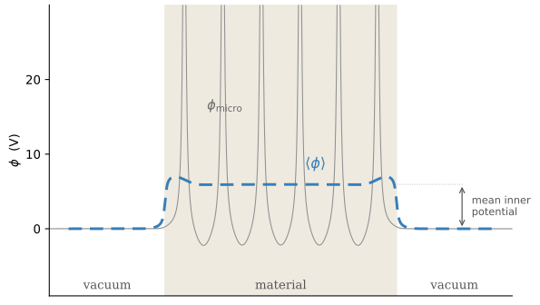
The microscopic potential in a material: violent spikes at the nuclear cores, wells in the bonds, all of it jiggling in time. Its running average rides flat across the interior at the mean inner potential, several volts above the vacuum outside.
The practical . Finally there is the that working electrochemistry actually pins down, which is defined through ion activity conventions; the prime is a reminder that it is one choice among many, since every activity convention defines its own. We met it in nonideal solutions: once a convention is adopted, is whatever value makes the bookkeeping come out, and it no longer corresponds to any physically-based electrostatic potential. It is a useful convention wearing 's notation, and we will come back to it. The parallel structure above also begs for a third Poisson equation: certainly one can take the Laplacian of and call the result a charge density , but what charge would that be? Nothing guarantees it is charge that exists. How the bookkeeping potential relates to real charge is a story that starts at the double layers below and finishes in the inhomogeneities topic.
Keeping the three separate already does a lot of work: the microscopic potential is real but unusable, the practical is usable but openly conventional, and all the interesting claims ride on in the middle. (Elsewhere in this book a bare appears only where the family members agree, or where their ambiguity is itself the topic; on this page the differences are the point, so the marks stay on.) So what does mean, for a particle? Exactly this:
The potential is the electrostatic energy per unit charge, of a hypothetical infinitesimally charged test particle that can permeate materials without disturbing them, and whose position is blurry enough to smear out the atomic-scale variations in the actual electric scalar potential.
That may sound like a quantity beyond any experiment, but the surprise is that this ghostly test particle very nearly exists. A fast electron in a transmission electron microscope crosses a thin specimen in around s, far too quickly to disturb it or be captured, and it flies straight through the core regions that real chemistry never visits, sampling the whole volume evenly. The phase of its wavefunction reads off the volume-averaged potential directly, and electron holographers routinely measure this mean inner potential : V in silicon, V in MgO, V in GaAs, V in PbS, and (closest to home for electrochemistry) V in liquid water.[3]
Notice the scale. The averaged potential inside a material sits far above the vacuum outside ( V even in liquid water, pushing V in dense crystals), positive because pointlike nuclei sit buried inside spread-out electron clouds,[4] while every energy difference in electrochemistry (electrode potentials, junction steps, overpotentials) plays out within a volt or two. So is real, and even measurable; it is the answer to a question about fast electron beams. What it is not, as we'll now see, is an ingredient in the energy of any thermalized ion or electron.
Real charges don't see
We want to know what an actual finitely-charged particle would see if placed in a material. Such a particle definitely disturbs the system, and its position will have correlations with other particles' positions. It is a mistake to say that is the electrostatic energy of a real ion or electron. Even to a very first approximation, the electrostatic potential felt by the particle would differ because:
- erroneously omits the local polarization of dielectric solvent and ionic atmosphere.
- erroneously includes the strong electric potentials around nuclear cores of surrounding particles. These are places that test charges go but real charged species do not.
And that is only a start. Of course, it may not even be possible to unambiguously specify such an idea as "electrostatic potential of an ion", as there is no sharp distinction between chemical bond and electric interaction. Sometimes is called the 'long distance part' of electrostatic energy, but even this is not correct since contains systematic long-distance errors.
And there is no experiment we can perform on the ions or electrons themselves that accesses : the mean inner potential is read out by fast beam particles, which are precisely the near-ideal test charges that no chemical species resembles. For the species we actually care about, is a poor approximation to anything, and an intangible one at that.
So what would be the right potential?
For a real charge, theory has several candidates, each constructed by asking what sits at an emptied site: the potential at the centre of an idealized Born cavity; the potential inside a cavity pushed open in the medium (close kin to the outer potential of a clean surface, up to curvature effects); or the potential at a site where a host and its electron cloud have been cut out of the frozen charge density.[5] These empty potentials are far better motivated than , since they at least ask what an arriving species would feel. But they are a family rather than a number: the continuum idealization, the relaxed cavity, and the frozen cut-out disagree with one another by surface-dipole terms of exactly the kind this chapter keeps meeting, and that residual arbitrariness is one more reason to keep the bookkeeping anchored to itself.
Chemists, it turns out, long ago built their own member of this family out of real ions. Tetraphenylarsonium () and tetraphenylborate () are a cation and an anion designed to be as close to identical twins as opposite charges allow: the same four phenyl rings in the same propeller arrangement, nearly the same size, each charge buried at the centre where no solvent molecule can reach it. Dissolve a trace of both in any solution and the midpoint of their two levels (at matched concentrations) is an honest observable: as real as any other level in this book, measurable down to partition ratios and concentration assays, defined wherever the twins dissolve. The famous TATB hypothesis is then not a measurement but a caption. It declares that no solvent can tell the twins apart, so that the midpoint may be read as 'the' potential of the solution, and its step across a solvent|solvent junction as 'the' Galvani potential difference; the standard single-ion transfer and hydration energy scales all descend from this one assumption.[6] Whether the caption is true is still contested; fittingly, the modern dispute turns on which other member of the empty-potential family the twins should be refereed against.
The internal chemical potential inherits the trouble
Let's go back to our electrochemical potential partitioning:
As discussed on the electrochemical potential tutorial, this does get rid of some annoying aspects of electricity like general arbitrary offsets. But since is a bad estimate of the electrostatic energy felt by an ion, that means must include all the necessary electrostatic corrections to . And that is in addition to any 'chemical-only' that might behave like an uncharged solute.
In principle this is fine, we can just say is an artificial number that shall compensate for all deficiencies in . But then, has no physical meaning: it is merely an artificial difference between two energies of different nature ( being a thermodynamic property of ions, being the electrostatic energy extrapolated from imaginary test charges that unnaturally permeate the material).
Really, does not deserve the name "chemical potential" since:
- it doesn't describe equilibrium between bodies (unless they perchance happen to have the same ).
- it is not any meaningful partial molar Gibbs energy (except in charge-neutral combinations of , such as ).
- is not even experimentally accessible, since is inaccessible to any measurement on the ions and electrons themselves.
Any consistent works equally well
The one benefit of is that it is at least consistently applied to all ions in the same place. This means that any local chemical reaction within a bulk solution, such as
looks the same in terms of the internal chemical potentials (since is the same for both ions):
But this would be satisfied by any random number in place of : the values would fully adjust to compensate for that too! As we saw in the case of nonideal solutions, that is precisely what happens when ion activity conventions are adopted: the practically used no longer corresponds to any physically-based electrostatic potential.
Galvani potentials and double layers
When we have two conductors made of different materials in direct contact, they will each internally have flat but there will be some step . Such a step corresponds to displaced positive and negative charges near the interface: on net (on the smoothing scale we use to establish ) there will be an overall nonzero electric field at/near the junction, and therefore a net step in . The step is a Galvani potential difference — the umbrella name for any such inner-potential step between two phases. The liquid junction potential is one special case of it: the step across a diffusing junction between two electrolyte solutions, held at zero current. A step between two metals in contact is a Galvani difference too, but never an LJP.
Let's be clear, the charge double layer is absolutely real. Our averages and do smudge out some of the details, but there truly is some kind of local charge displacement and electric field. What is questionable is its importance: only a test charge would perceive the complex interface as a mere electric double layer, and for any real ion, the energy difference that it experiences is not going to be . The double layer may be physically real, but it is mostly a distraction from what we actually care about.
For example, between a metal and semiconductor, or between two distinct semiconductors (like AlGaAs and GaAs), we really care about the relative positions of Fermi levels and the semiconductors' conduction bands . Not only that, we care about the detailed structure inside of the junction (the band bending, and the atomic jump). All of this can be addressed without ever talking about the infinitesimal test charge's .
When it comes to electrolytes, we can ask what the double layer (or ) is at the interface of a water-based solution and a benzene-based solution. But that is not what we care about, and indeed is totally unmeasurable here. Instead we want to analyze equilibration of (electro-) chemical potentials, and we also care about the ionic diffuse layer ("band bending").
A step made of nothing
Just how disconnected the Galvani step can be from anything an ion experiences is easiest to see in a thought experiment. Imagine two solvents, hillium and mountainium, engineered to be chemically identical: the same valence electron structure, the same dielectric response, the same solvation of every solute. They differ only in the architecture of their deep, inert atomic cores, which are smooth and smeared-out in hillium but compact and spiky in mountainium. Fill the left half of a vessel with one and the right half with the other, dissolve some salt throughout, and let everything equilibrate.
Since no ion can tell the two solvents apart, nothing happens at the interface: the concentrations stay uniform, every and the whole ladder run dead flat across the junction, no double layer forms, and the physical displacement field is zero everywhere.
Now compute . Deep in each bulk it is flat, but the two flat values differ: a pointlike core buried in its electron cloud raises the volume average more than a smeared-out one does, even though (by Gauss's law) the two produce identical fields outside the core region, which is exactly why no solute could tell them apart. So takes a step at the interface, quite possibly of several volts, of the same nature as the mean-inner-potential offsets measured above. There is our Galvani potential difference: a step between two liquids that no solute can distinguish, made entirely out of core architecture. No charge moved to create it, no ion feels it, and no experiment on the solutes could ever find it.[7] The practical , meanwhile, rides at a fixed offset from the ladder (that is what an activity convention pins), so it runs dead flat through the junction: here the bookkeeping potential is more faithful to what the ions experience than the honest average is. (The empty potentials from earlier likewise sail through flat, since they sample the medium only from outside the core radii; the step belongs to alone.)
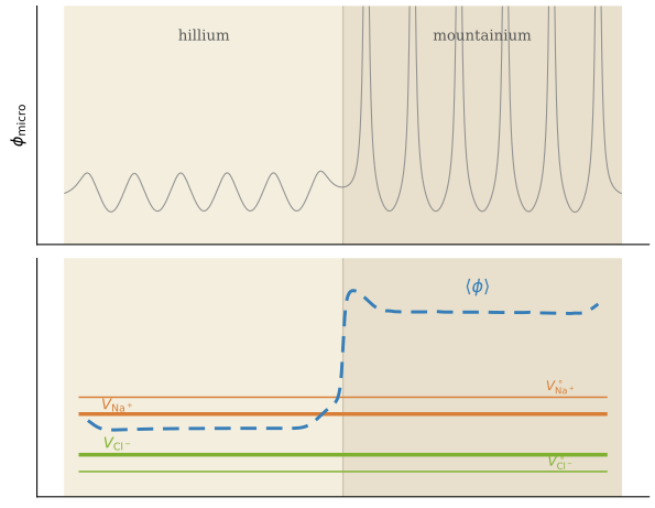
Hillium and mountainium: two solvents identical to every solute, differing only in core architecture. Top: , gentle on the left, spiky on the right. Bottom: steps at the junction while the ladder and every run dead flat. The Galvani step is made of core shape, and no ion feels it.
Where genuinely works, and why
The hillium picture also explains where works honestly. Between two regions of the same medium (the same semiconductor with different doping, say, or the same dilute solvent with different salt content), the core-architecture contributions to the average are identical on both sides and cancel out of . What remains of the step faithfully tracks the differences in the meaningful energy levels, like the conduction band edge or the ionic standard states . This is the regime behind every success of : band bending, Debye screening, Donnan steps, built-in potentials. Indeed, the same electron holography that reads the mean inner potential can map the built-in step across a silicon p-n junction, and it finds the expected volt or so,[8] precisely because both sides are the same crystal and the core-architecture offset drops out of the difference. Within one medium, following is the same thing as following the ladder, and no harm comes of it. This is also the regime where the third Poisson equation becomes meaningful: the equation that basic electrostatics runs on the ladder is in effect a Poisson equation with the real screening charge as its source.
You can say that "the corrections to become small in this case", but I would rather say that in this case mimics the energy differences that actually matter. The distinction bites as soon as the two sides are not the same medium. A salt bridge, for instance, is routinely presented as "shorting together" two solutions' values as naturally as shorting together two wires; in reality, as discussed in Basic transport, its minimization of the junction step is a complicated nonequilibrium phenomenon that relies on identical solvents and on correctly selected salts that dominate the diffusion. The picture quietly fails for different solvents, and even for nonideal solutions of the same solvent.
The semiconductor community learned the same lesson within its own borders. Introductory teaching leans on the "built-in potential" of the p-n junction, which works because both sides are the same crystal. Then come heterostructures and graded junctions, where stops mattering at all: what truly matters is how the bands are bending.
Inner potentials of metals
With semiconductors or electrolytes, the notion of is at least helpful as a naive explanation of things like band bending or salt bridges. But in metals there is no significant band bending, and the concept of an inner potential is simply dubious.
One problem is with voltmeters: if we want to say that voltmeters measure , then we have to make sure all our unnecessary metal potentials cancel out. The common practice is to conceptually "bookend" our device's electrodes with two metals of identical composition, so that happens to agree with the voltage difference . For example, the following figure:
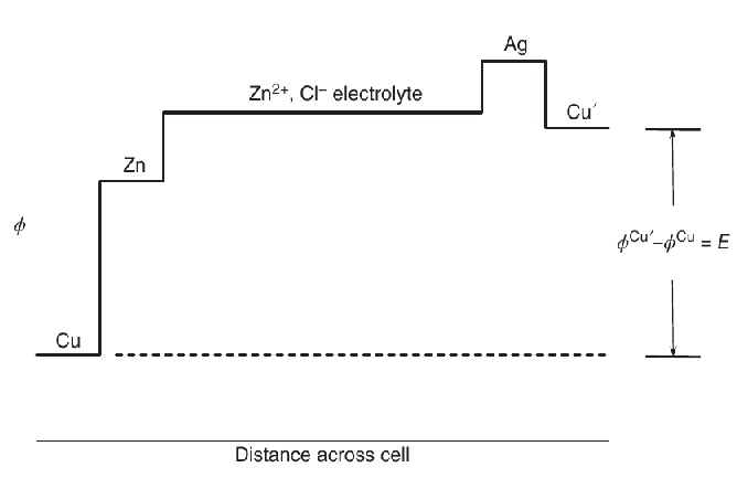
Profile of across a device, as relating to measured voltage . From Bard & Faulkner's Electrochemical Methods (2022) Fig 1.1.2 (fair use reproduction).
Unlike a proper band diagram, a plot of vs position is cluttered by the matching-metal bookends and all sorts of extra Galvani potentials between metals. A pragmatic electrochemist will soon sweep this tedious visualization under the rug and thereafter focus on the math of electrode potentials.
Another problem relates to the double layers: where a metal meets a non-metal (semiconductor or electrolyte), there is a near-discontinuous (angstrom-scale) jump in just at the surface, that is going to depend nontrivially on the nature of the other material, followed by a smoother region where approaches its equilibrium value more gradually (band bending). Thus we actually have a triple layer. Although we can do all sorts of experiments probing the gradual- region (again, since bending corresponds to bending of relevant energy levels!), we are never able to do an experiment that relates to the abrupt jump, i.e., we never probe the full triple layer. The only potential of a metal that enters is , or Fermi level.[9]
Two doors out
If is ambiguous, then in places so is , the electric field that is supposed to be objective. Surprisingly, Maxwell's equations take no offense: they lean only on the curl of and on , and both survive the ambiguity untouched. That story really belongs to inhomogeneous media, so it gets its own topic, the one after next.
The other natural exit is outward. Just outside any surface, in the vacuum, sits a potential that is unambiguous, honestly measurable, and free of every complaint raised on this page, and it is tempting to anchor everything to it. How far that actually carries is the next topic.
Before that, a closing word to the theoretical and computational electrochemists. In a simulation comes nearly for free (smoothing recipes exist), and it can even be advantageous as a control variable. But a computed is still the mean inner potential: report energies referenced to it (or set and leave results unreferenced) and your numbers are tied to the arbitrary shape of the inert cores, as the holography values above make vivid. Indeed, a pseudopotential calculation re-enacts hillium and mountainium by construction: it swaps each spiky core for a smooth one that produces the same potential outside a small cutoff radius, so the chemistry is preserved while the computed average shifts, and the such a code reports is the mean inner potential of its smoothed stand-in material, not of yours. (The calculations that match the holographic values are, accordingly, all-electron ones.[10]) Computing that average correctly is delicate in its own right; the measured water value came out larger than most quantum-simulation predictions. The quantities worth the extra effort are the electrochemical potentials , since they are what the ions and electrons actually experience; output differences of those, and comparison with experiment, and between codes, becomes direct.
Takeaways
"The electrostatic potential" of a material names three different things. The microscopic potential is real and violently structured, and no one disputes it. Its smoothed average is also real, and even measurable (a mean inner potential of several volts, read out by fast electron beams), but it answers a beam-physics question: for thermalized ions and electrons, estimates nothing, and the partitioning of into is "without physical significance", as Guggenheim said a hundred years ago. And the practical of working electrochemistry is a bookkeeping convention, pinned by ion-activity choices rather than by electrostatics.
Where seems to work (band bending, built-in potentials, salt bridges between like solutions), it is because within one medium the step in mimics the step in the ladder, and the ladder is the part that matters. The electrochemical potentials are the quantities thermodynamics actually provides, and voltmeters measure .
I hope that the species voltage and its associated visual band diagrams will help promote this -less approach and bring together the semiconductor and electrochemical communities into a unified viewpoint.
For a modern defence and sharpening of that thesis, see B. A. Pethica, Are electrostatic potentials between regions of different chemical composition measurable? The Gibbs–Guggenheim principle reconsidered, extended and its consequences revisited, Phys. Chem. Chem. Phys. 9, 6253 (2007). ↩︎
It is also subject to gauge ambiguity with the magnetic vector potential; as usual we invoke the "electrostatic approximation", in which the electric field curl is negligible and the potential is the anti-gradient of the electric field. ↩︎
Crystals: M. Gajdardziska-Josifovska, M. R. McCartney, W. J. de Ruijter, D. J. Smith, J. K. Weiss and J. M. Zuo, Accurate measurements of mean inner potential of crystal wedges using digital electron holograms, Ultramicroscopy 50, 285 (1993); further III-V values in P. Kruse, A. Rosenauer and D. Gerthsen, Determination of the mean inner potential in III-V semiconductors by electron holography, Ultramicroscopy 96, 11 (2003). Liquid water: M. N. Yesibolati, S. Laganà, H. Sun, M. Beleggia, S. M. Kathmann, T. Kasama and K. Mølhave, Mean inner potential of liquid water, Phys. Rev. Lett. 124, 065502 (2020). For the technique itself: R. E. Dunin-Borkowski, T. Kasama and R. J. Harrison, Electron holography of nanostructured materials, in Nanocharacterisation (Royal Society of Chemistry, 2007). ↩︎
More precisely it reflects the full microscopic charge density: the value is exquisitely sensitive to how bonding redistributes the valence charge, and it cannot be pinned down from X-ray diffraction data alone. M. O'Keeffe and J. C. H. Spence, On the average Coulomb potential () and constraints on the electron density in crystals, Acta Cryst. A 50, 33 (1994). ↩︎
The last is the "empty potential" of R. T. Tung's host–bath analysis: Energy Level Alignment of Solid Interfaces (World Scientific, 2026), ch. 1. The construction appears already in his earlier review, The physics and chemistry of the Schottky barrier height, Appl. Phys. Rev. 1, 011304 (2014), where Fig. 22 defines the empty potential by cutting a few cells' charges out of a crystal. ↩︎
The twins are chemistry's answer to the cut-out construction: rather than theorize the cavity, build two of them, identical except for the sign. The hypothesis underwrites the recommended single-ion tables: Y. Marcus, Thermodynamic functions of transfer of single ions from water to nonaqueous and mixed solvents: Part 1, Pure Appl. Chem. 55, 977 (1983); and C. Kalidas, G. Hefter and Y. Marcus, Gibbs energies of transfer of cations from water to mixed aqueous organic solvents, Chem. Rev. 100, 819 (2000), who state the epistemics plainly: such assumptions can be checked for self-consistency, but "their correctness (accuracy) cannot be determined." Extended (conditionally: "if it is accepted as applying to the hydration of ions…") to transfers from the gas phase, it yields the 'absolute' single-ion hydration energies: Y. Marcus, The thermodynamics of solvation of ions. Part 4, J. Chem. Soc., Faraday Trans. 1 83, 2985 (1987). Operationally the twins are a probe rather than a bridge: measure how the pair partitions between two solvents, split its transfer energy evenly, and by salt additivity every other ion's transfer follows — the on-paper splitting that stretches single-ion scales (electrode potentials, pH) across the solvent divide. Molecular simulation begs to differ — water hosts the anion more happily, its hydrogens reaching into the phenyl seams: R. Schurhammer and G. Wipff, Are the hydrophobic AsPh₄⁺ and BPh₄⁻ ions equally solvated?, J. Phys. Chem. A 104, 11159 (2000). But how much of the telling-apart is physics rather than convention itself depends on the reference cavity: compare, in one and the same journal issue, T. T. Duignan, M. D. Baer and C. J. Mundy, Understanding the scale of the single ion free energy, J. Chem. Phys. 148, 222819 (2018), who conclude the assumption should be abandoned, with T. P. Pollard and T. L. Beck, Re-examining the tetraphenylarsonium/tetraphenylborate (TATB) hypothesis, J. Chem. Phys. 148, 222830 (2018), who find most of the computed asymmetry is the cavity-potential convention, with a residue that is small in water and DMSO but genuine in low-polarity solvents. The standing ≈0.4 V disagreement between TATB-based and cluster-based single-ion scales is surface-dipole ambiguity of exactly the same kind that separates the theoretical family members above. ↩︎
Its precise size even depends on the choice of smoothing recipe, a point that will return in the inhomogeneities topic. ↩︎
M. R. McCartney, D. J. Smith, R. Hull, J. C. Bean, E. Voelkl and B. Frost, Direct observation of potential distribution across Si/Si p-n junctions using off-axis electron holography, Appl. Phys. Lett. 65, 2603 (1994). ↩︎
The potentials of metals can actively mislead, too. A long-standing myth attributes thermoelectric voltages to junctions, via the temperature dependence of Galvani potentials (or of contact potentials, as illustrated here). In fact the thermoelectric voltage develops as a gradient of only in the regions of thermal gradient, and takes no step at the junction itself. A correct account can be forced through or or , but every extra reference level must then be dragged through the thermal gradients only to cancel back out of the final answer; see Apertet et al. (2016), "A note on the electrochemical nature of the thermoelectric power". ↩︎
P. Kruse, M. Schowalter, D. Lamoen, A. Rosenauer and D. Gerthsen, Determination of the mean inner potential in III–V semiconductors, Si and Ge by density functional theory and electron holography, Ultramicroscopy 106, 105 (2006): full-potential LAPW slab calculations reproduce the holographic Si and GaAs values, and land about 10% below isolated-atom estimates because bonding redistributes the charge. ↩︎